julian • Dec 16, 2025

Advent of Code Quantum Edition: Day 2

Advent of Code 2025 Day 2, quantum edition: use QFT in Qiskit to detect repetition via frequency spikes, then unpack why input state preparation limits speedups on Aqora.

Summarize with AI

🚨 spoilers 🚨 for the advent of code day 2. If you’d rather not be spoiled, please do not read any farther

Welcome to Day 2 of me trying procrastinate on my “regular ol’” software engineering job, by coming up with complicated quantum solutions to the daily Advent of Code challenges. If you haven’t read the last day’s post, I would recommend you read it, not just because my ego demands it, but because it provides a good basic understanding of quantum circuits, qiskit and what’s the reason for doing this all in the first place. I am excited however, because in contrast to the last post, Day 2 will provide us with some good opportunities to actually explore some quantum effects. But before we get ahead of ourselves, let’s look at the problem, and what a classical solution might look like.

The Boring Way

Like before, Eric is way better at setting up his problems than I am, so I would highly recommend you read the description of Day 2, but in brief, the problem is as follows: Let

N

be a positive integer with

n

digits. Determine whether

N

can be written as a repetition of a smaller integer. That is, decide whether there exists an integer

k

with

0 < k \leq n/2

and a

k

-digit integer

d

such that the decimal representation of

N

is obtained by repeating the digits of

d

exactly

n/k

times. So that

N = \underbrace{dd \cdots d}_{n/k \text{ times}}

We can do this quite easily classically. We just have to check all

d

where

d

is the first

k

digitis of

N

where

0 < k \leq n/2

and check to see if

N

is a repetition of

d

. So I’ve thrown together the python implementation below

def iter_chunks(item: int, size: int):
    base = 10 ** (size)
    while item > 0:
        yield item % base
        item //= base

def check(item: int):
    length = len(str(item))
    for i in range(1, length // 2 + 1):
        if length % i != 0:
            continue
        if all_equal(iter_chunks(item, i)):
            return True

So it’s pretty good as is! We have two loops here one to iterate over

k

digits and one to check if the repetition is equal. So that falls plainly in our P problem space with

O(n^2)

but can we do better with quantum?

The Fast and the Fouriers

Looking at this problem, what stands out to me is the repetition here. Things that repeat have a certain frequency to them, so if we are able to translate the inputs to this problem into a frequency domain, maybe we can analyze the frequencies to see if there exists a strong signal we can check. For example let’s look at the following signal

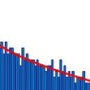
We can clearly see repetition. There appears to be 5 larger chunks and within those 5 chunks we can see a smaller wave form that repeats itself, we can sit here and count the peaks and troughs, but it’s hard to analytically figure out the structure of the signal. If we translate this signal from the “Natural Domain” to the “Frequency Domain” we can maybe have more insight on the underlying structure. To do this we can use the Fourier Transform. I’m using a pseudo Fourier Transform below from the very good 3 Blue 1 Brown Visual Explanation because I think it’s more clear how to map from the natural domain to the frequency domain.

Here we can clearly large spikes at the frequencies 5, 15 and 30. And indeed I constructed the signal above by adding 3 sine waves of frequency 5, 15 and 30 together.

Fourier transforms are fantastic tools for analyzing repetition. But so far we’ve been looking at analog signals, but classical computers are digital and discrete. For that we would need a discrete Fourier transform or DFT (not to be confused with Density Functional Theory which unfortunately will probably not come up in the Advent of Code this year, but you never know 🤞). DFT treats a digital signal as a sampled wave and can perform the same frequency analysis.

Fantastic! So for our

N

with digits

d_0, d_1, ... d_{n-1}

we can treat

d_t

as the amplitude of a wave at time

t

and then we can use DFT to find any repetition in our wave. Unfortunately DFT is

O(n^2)

😢 but there exists a Fast Fourier Transform or FFT which is equivalent to DFT which can run in

O(n \log n)

🥲 Can quantum computers do any better?

Quantum Fourier Transform

You guessed it! The hottest FT since NFT’s, it’s the Quantum Fourier Transfer or QFT. QFT is quite simply the quantum analog to DFT, and work in a very similar way. Which might make us pose the question: how does DFT work? Like I’ve mentioned before 3 Blue 1 Brown gives a very good intuitive understanding of how a Fourier transform operates (and if you’d like to take it one step further and understand the math more, the video on Laplace transforms, of which the Fourier transform a special case taken along the imaginary axis, is a good guide) but to put it very simply, the transform takes in a set of functions and returns a set of exponential functions that describe that function. For example DFT’s definition is as follows:

X_{k}=\sum _{n=0}^{N-1}x_{n}\cdot e^{-i2\pi {\tfrac {k}{N}}n}

Now, if you’re like me, you get a little bit scared when you see an equation like this with

e

’s and

i

’s, but the important thing is to remember euler’s formula, or rather that

e^{i \phi}

where

\phi

is an angle in radians, just represents a rotation around the unit circle.

There’s lots of good explanations for this, so I’m not going to elaborate more here (I’d refer you again to 3 Blue 1 Brown, I think he’s done it a few times in different ways). With that in mind we can look back on the DFT formula and see that given a sequence of numbers

X_k

we’re breaking it down into different rotational elements. See how the phase

\phi = 2\pi {\tfrac {k}{N}}n

is just different fractions of a full rotation. The quantum Fourier transform works along the same lines. In fact it’s equation can be written almost identically

X_{k}= {\tfrac {1}{\sqrt {N}}} \sum _{n=0}^{N-1}x_{n}\cdot e^{i2\pi {\tfrac {k}{N}}n}

The only difference is that quantum computers can represent these complex numbers more naturally

Superposition 🦸

As we saw in the previous day, we can represent 0 and 1’s quite easily with qubits and do logic operations on them. We often look at the individual state of a qubit as a Bloch sphere where the

\ket{0}

state is on the top and the

\ket{1}

state is on the bottom

The benefit of the Bloch sphere is that we can also look at states of the qubit that are a superposition between

\ket{0}

and

\ket{1}

. For example the state

\tfrac{1}{\sqrt{2}}\ket{0} + \tfrac{1}{\sqrt{2}}\ket{1}

We can’t observe these “in-between” states directly without them collapsing into either a

\ket{0}

or a

\ket{1}

. The state above, for example, has an equal 50/50 chance of either collapsing into a

\ket{0}

or a

\ket{1}

when we go to measure it. In fact, any state along the “equator” of the qubit, has this 50% chance. So for all intents and purposes, any state rotated around the the pole of the qubit, or the Z-axis, along its equator are the same to us when measured. However, this rotation around the Z-axis can give quantum computers some truly extraordinary super powers. We call the angle of the rotation around the Z-axis the phase of the qubit, and it lies at the heart of QFT.

How QFT works

If we go back to the definition of QFT

X_{k}= {\tfrac {1}{\sqrt {N}}} \sum _{n=0}^{N-1}x_{n}\cdot e^{i2\pi {\tfrac {k}{N}}n}

We’ll remember the QFT breaks down a set of numbers into a fractional set of rotations. To encode this set of rotations, we will use the phase of the qubit. From the Qiskit documentation, we can see how we encode a 4 qubit system from its quantum computational basis

to it’s quantum fourier computation basis

To build this using a circuit is actually quite straight forward. We will use something called a controlled RZ gate. If you recall from day 1, a controlled NOT gate, or CNOT gate, has a control qubit and a target qubit. If the control qubit is

\ket{1}

it will flip the target qubit state. In the case of the CNOT gate this is done by rotating it around the X-axis of the qubit. With a controlled RZ gate, we set a control qubit and a target qubit in the same way, but this time if the control qubit is

\ket{1}

then the target qubit is rotated around the Z-axis by a defined amount. We can use a set of create our quantum fourier transform!

To break this down, for each qubit, starting from the bottom, we first put the qubit into a superposition using the Hadamard gate, the orange H gates you see. For right now all you need to know about the Hadamard gate is that it’s a good way to put a qubit into a superposition state (e.g. that 50/50 state that we looked at before). Then for each qubit above, we apply a controlled Z rotation, by increasing fractions. In that way we can additvely achieve the different phases for each qubit that we see in the the quantum fourier computation basis. Now let’s see it in action!

Finally some Quantum Computing

Let’s get our fingers warmed up and plug in the quantum computer. We’re finally going to code a quantum algorithm. Our problem looks like this. We want to see if the following string has a repetitive substring in it

classical_string = [1, 2, 3, 4, 5, 1, 2, 3, 4, 5, 1, 2, 3, 4, 5]

The astute among you will notice, that it’s just the numbers 1-5 repeated 3 times, but we will let our quantum computer be the final judge! First we will need to encode the string in a way that the quantum computer will understand. We do that by initializing the qubits, to the probability of measuring them. The higher the number, the higher the probability of measuring it. We can do that with the following snippet

N = len(classical_string)

# get the number of qubits: log2(N)

qubits = N.bit_length()

# pad the amplitude vector

amplitude_vector = classical_string + classical_string[:2**qubits - N]

# normalize the amplitudes

normalized_amplitudes = amplitude_vector / np.linalg.norm(amplitude_vector)

# create our circuit

qc = QuantumCircuit(qubits)
qc.initialize(normalized_amplitudes, qc.qubits)

First we need to create our amplitude vector and normalize it. We first calculate the number of qubits required to represent it, we have 15 numbers, so the next power of 2 is 16 and we’ll need 4 qubits. We can pad the remainder of the amplitude vector with our string repeated, as it is hopefully a repeating string, and normalize the amplitudes so that the probabilities will add up to 1. We can then use Qiskit to initialize a circuit with those probabilities. We can sample the circuit to verify

Perfect! We can already see that discrete wave like pattern that DFT would process. So now all that’s left to do is run it through our QFT! We’ve already constructed it above, but qiskit provides the exact same gate as part of its circuit library so we’ll just pop it in.

qc.append(QFTGate(len(qc.qubits)), qc.qubits)

And we can go ahead an sample it!

Hmmm, okay, that doesn’t seem very helpful, maybe if we remove the

0000

bin (as its a trivial solution to a repetition problem) from the graph it will be more clear

Okay, now we can see larger spikes at 3 and 13 and two smaller spikes at 6 and 10, but to be honest this still doesn’t tell us very much 😞 Maybe there’s not enough repetition? Let’s try scaling up our problem and repeating our string longer

classical_string = [1, 2, 3, 4, 5] * 102

Now our string is 510 digits long, and we have

log_2512=9

qubits to play with! Let’s measure it

Okay now we have some very well defined spikes. It’s hard to see from the plot, but our spikes are located at 102, 205, 307 and 410. If you notice, those numbers are quite evenly spaced with a spacing of around 102 or 103. In fact… 🤔

512/102.5 = 4.99512195122 \approx 5

We did it! We found our substring size! And if we look at our earlier graph, we can see a spacing of a little greater than 3 in our space of 16, so we will get a similar approximation of 5. The more analytical way of deriving this number is by using continued fractions, but I think this is good enough for now

Did we beat the classical solution

Let’s try to analyze the time complexity for our quantum solution. If we look back at our QFT circuit that we built, we’ll notice that for a QFT gate with

n

qubits, for each qubit we will have to do at most

n

controlled RZ gates. Which means that our QFT gate runs in

O(n^2)

time. However, because we were able to encode 15 numbers into 4 qubits, our number

N

is actually reduced to size

\log_2N

which means that our time complexity is actually

O((\log n)^2)

! We did it! Quantum advantage achieved!

Oh well 👉👈 there’s one thing I forgot to mention. Do you remember that little snippet of code that I breezed over

qc.initialize(normalized_amplitudes, qc.qubits)

Well it turns out initializing a quantum state isn’t that easy 😅 The best known circuits for initializing an arbitrary quantum state as far as I know is

O(2^n)

which isn’t great at all. If we had these states in quantum RAM or similar, this may be useful, but as it is, it’s not very useful at all. In addition, we can’t forget that he number of measurements required to sample from our circuits also scale with

N

so in reality our algorithm is more like

O(n(\log n)^2)

So is any of this useful???

Maybe not today, but it will be very useful in the future! Maybe you’ve already heard of Shor's algorithm, but if you haven’t, Shor’s algorithm can factor numbers in

O((\log N)^{2}(\log \log N))

whereas the classical factoring tends to do it in

O(e^{1.9(\log N)^{1/3}(\log \log N)^{2/3}})

and if you’re keeping track, that’s making an exponential problem a polynomial problem, so for large numbers instead of taking millenia, it could take a few seconds. And low and behold, at the heart of Shor’s algorithm lies QFT and trying to find a period (or cycles of repetition) for a function relating to the factors of a number.

But for right now, its useful as a learning tool, and maybe it’s helped me at the minimum to broaden my understanding of classical algorithms such as DFT. And we will continue our quantum quest for Day 3 soon! See you then!!!